7 Strategic Capacity Planning

Learning Objectives
- What are common capacity strategies?
- Calculate efficiency and utilization measures.
- Describe factors that determine effective capacity.
- Understand the steps in the capacity planning process.
- Determine the capacity in a sequential process with a bottleneck.
- Use break even analysis to evaluate capacity alternatives.
This module examines how important strategic capacity planning is for products and services. The overall objective of strategic capacity planning is to reach an optimal level where production capabilities meet demand. Capacity needs include equipment, space, and employee skills. If production capabilities are not meeting demand, it will result in higher costs, strains on resources, and possible customer loss. It is important to note that capacity planning has many long-term concerns given the long-term commitment of resources.
Managers should recognize the broader effects capacity decisions have on the entire organization. Common strategies include leading capacity, where capacity is increased to meet expected demand, and following capacity, where companies wait for demand increases before expanding capabilities. A third approach is tracking capacity, which adds incremental capacity over time to meet demand.
Finally, the two most useful functions of capacity planning are design capacity and effective capacity. Design capacity refers to the maximum designed capacity or output rate and the effective capacity is the design capacity minus personal and other allowances. These two functions of capacity can be used to find the efficiency and utilization. These are calculated by the formulas below:
Efficiency = (Actual Output / Effective Capacity) x 100%
Utilization = (Actual Output / Design Capacity) x 100%
Effective Capacity = Design Capacity – allowances
Example
Actual production last week = 25,000 units
Effective capacity = 28,000 units
Design capacity = 230 units per hour
Factory operates 7 days / week, three 8-hour shifts
- What is the design capacity for one week?
- Calculate the efficiency and utilization rates.
Solution
(Using the formulas above)
- Design capacity = (7 x 3 x 8) x (230) = 38,640 units per week
- Utilization = 25,000 / 38,640 = 64.7%
Efficiency = 25,000 / 28,000 = 89.3%
Capacity Planning for Products and Services
Capacity refers to a system’s potential for producing goods or delivering services over a specified time interval. Capacity planning involves long-term and short- term considerations. Long-term considerations relate to the overall level of capacity; short-term considerations relate to variations in capacity requirements due to seasonal, random, and irregular fluctuations in demand.
Excess capacity arises when actual production is less than what is achievable or optimal for a firm. This often means that the demand in the market for the product is below what the firm could potentially supply to the market. Excess capacity is inefficient and will cause manufacturers to incur extra costs. Capacity can be broken down in two categories: Design Capacity and Effective Capacity.
Three key inputs to capacity planning are:
- The kind of capacity that will be needed
- How much capacity will be needed?
- When will it be needed?
Defining and Measuring Capacity
When selecting a measure of capacity, it is best to choose one that doesn’t need updating. For example, dollar amounts are often a poor measure of capacity (e.g., a restaurant may have capacity of $1 million of sales a year) because price changes over time necessitate updating of that measure.
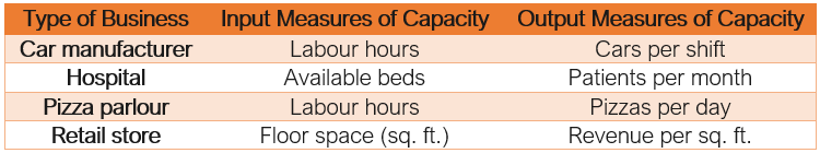
When dealing with more than one product, it is best to measure capacity in terms of each product. For example, the capacity of a firm is to either produce 100 microwaves or 75 refrigerators. This is less confusing than just saying the capacity is 100 or 75. Another method of measuring capacity is by referring to the availability of inputs. This is usually more helpful if we are dealing with several type of output. Note that one specific measure of capacity can’t be used in all situations; it needs to be tailored to the specific situation at hand. The following table shows examples of both output and input used for capacity measures.
Determinants of Effective Capacity
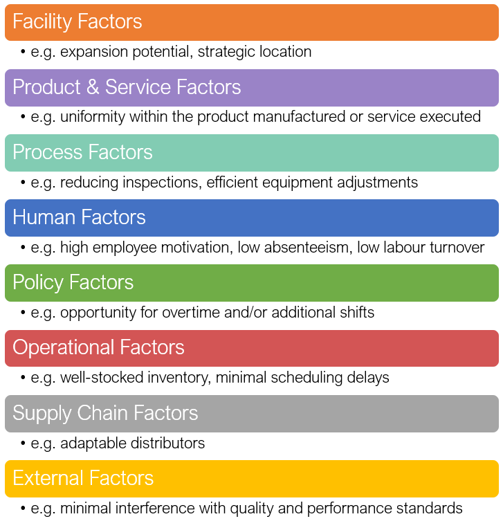
- Facilities: The size and provision for expansion are key in the design of facilities. Other facility factors include locational factors, such as transportation costs, distance to market, labor supply, and energy sources. The layout of the work area can determine how smoothly work can be performed.
- Product and Service Factors: The more uniform the output, the more opportunities there are for standardization of methods and materials . This leads to greater capacity.
- Process Factors: Quantity capability is an important determinant of capacity, but so is output quality. If the quality does not meet standards, then output rate decreases because of need of inspection and rework activities. Process improvements that increase quality and productivity can result in increased capacity. Another process factor to consider is the time it takes to change over equipment settings for different products or services.
- Human Factors: the tasks that are needed in certain jobs, the array of activities involved, and the training, skill, and experience required to perform a job all affect the potential and actual output. Employee motivation, absenteeism, and labour turnover all affect the output rate as well.
- Policy Factors: Management policy can affect capacity by allowing or disallowing capacity options such as overtime or second or third shifts
- Operational Factors: Scheduling problems may occur when an organization has differences in equipment capabilities among different pieces of equipment or differences in job requirements. Other areas of impact on effective capacity include inventory stocking decisions, late deliveries, purchasing requirements, acceptability of purchased materials and parts, and quality inspection and control procedures.
- Supply Chain Factors: Questions include: What impact will the changes have on suppliers, warehousing, transportation, and distributors? If capacity will be increased, will these elements of the supply chain be able to handle the increase? If capacity is to be decreased, what impact will the loss of business have on these elements of the supply chain?
- External Factors: Minimum quality and performance standards can restrict management’s options for increasing and using capacity.
Inadequate planning can be a major limitation in determining the effective capacity.
The most important parts of effective capacity are process and human factors. Process factors must be efficient and must operate smoothly. If not, the rate of output will dramatically decrease. They must be motivated and have a low absenteeism and labour turnover. In resolving constraint issues, all possible alternative solutions must be evaluated.
- Estimate future capacity requirements
- Evaluate existing capacity and facilities and identify gaps
- Identify alternatives for meeting requirements
- Conduct financial analyses of each alternative
- Assess key qualitative issues for each alternative
- Select the alternative to pursue that will be best in the long term
- Implement the selected alternative
- Monitor results
The above content is an adaptation of Saylor Academy’s BUS300 course.[1]
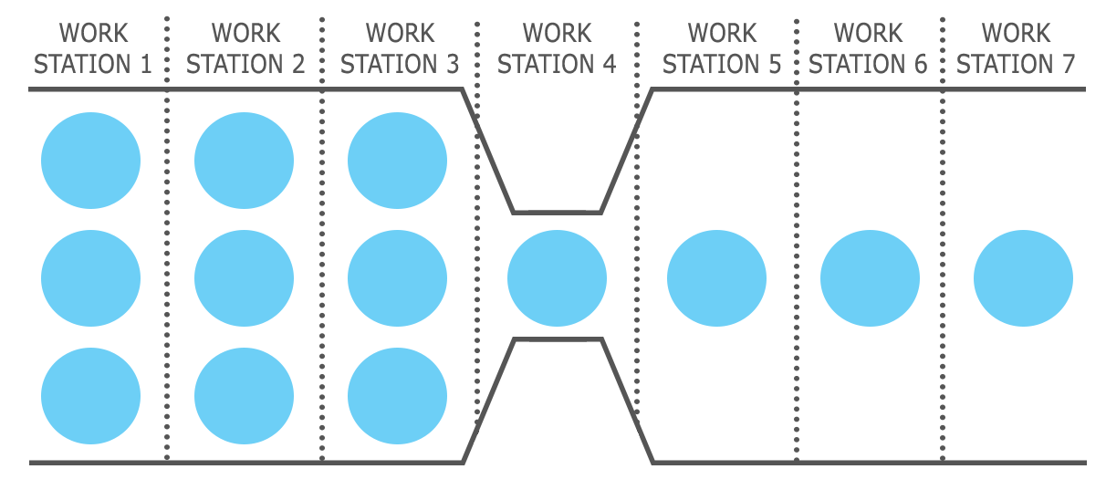
The Sequential Processes and the Bottleneck
Any process that has several steps, one after another, is considered a sequential process. A good example of these processes is the manufacturing assembly line in which each workstation gets inputs from a previous workstation and give its outputs to the next workstation. It is safe to assume that each step has its own staff member, since this is exactly what happens in assembly lines. For this kind of process, it is crucial to have a balanced time across all steps. That is, there should not be any big difference between the amounts of time that different steps take to process one unit of product. For example, if step 1, 2 and 3 take 3, 10 and 5 minutes consecutively to process one unit of product, two main issues will happen during the production:
1) There will be a big pile of inventory sitting right before step 2, since step 1 is much faster than step 2, and the products that are already processed in step 1 will need to wait for step 2 to be done with its current unit at hand. As a result, this becomes an inventory holding issue, which is costly.
2) Step 3 will always need to wait for step 2 for an extra 5 minutes. This is due to the fact that step 3 finished its current product at hand in 5 minutes, but step 2 needs a total of 10 minutes to finish its work and feed it to step 3. This causes step 3 to be idle for a long time, which is also costly for the company. This is costly, because the company is already paying the staff who works in step 3 for the whole time, but they are not able to produce as many units as they should due to the very slow entry of the inputs coming from step 2.
The bottleneck is the slowest step in each process or the slowest process in a system. The capacity of the bottleneck defines the capacity of the whole process. In our example above, step 2 was the slowest, and as a result, the bottleneck. This means that the whole process (including all steps 1 to 3) will not be able to have an output any faster than one every 10 minutes. In the following, let’s see why this is happening:
In an 8-hour shift per day, we have 8 x 60 = 480 minutes
Assuming that step 1 has enough input to process during the day, the total output from step 1 will be 480 / 3 = 160 units per day. This is the capacity for step 1. In a similar way, the capacity for step 2 is 480 / 10 = 48, and the capacity for step 3 is 480 / 5 = 96 units.
This means that the input to step 2 will be 160 units to be processed. But as we see, step 2 will only be able to process a maximum of 48 units per day. That means that only 48 units get to step 3 for processing. Since step 3 has a capacity of 96 units per day, it will easily process those 48 units of inputs, and the output from step 3 will be 48 units. Because the step 3 is the last step of our process, this output of 48 units will automatically be the total output of the whole process per day.
The key observation here is that the capacity of step 2, which is the bottleneck, determined the capacity of the whole process. This concept is very important in practice. Often times, the companies that do not pay attention to the concept of bottleneck and its implications invest in parts of the process that are not bottleneck. This will keep the bottleneck unchanged and as a result, they will not see any improvement in the capacity of the whole process.
Example
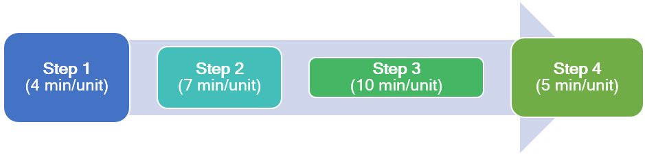
Caroline has a thriving business selling her tote bags through several popular websites. Her business volume has caused her to hire full-time employees. Her business has four main manufacturing operations: 1) cutting fabric (4 min), 2) stitching fabric (7 min), 3) adding zippers, toggles, and liner (10 min), and 4) inspecting, packing, and labeling (5 min).
Employees work 7 hours per day. Help Caroline to determine the following:
- Based on her very high demand, is there a bottleneck and what stage is it? What is the capacity of the process per day?
-
Caroline’s employee at step #2 has found a new machine that will enable him to do the stitching faster, at a rate of 5 min per bag instead of 7 min. The machine costs $3500. Would you suggest this is a good investment to help Caroline increase her output? Why or why not?
- If there were another person to be added to the process, where should Caroline add him or her and what would be the new capacity?
Solution
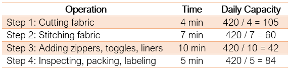
(Based on 7×60 = 420 min per day)
Accessible format for Figure 4.4
- The maximum output is 42 units, because that is what the bottleneck can do. The bottleneck is at stage #3, which is the slowest part of the process.
- Caroline should NOT invest any funds into step #2. This may speed up the stitching, but the maximum output of the process will still be 42 units because step #3 has not changed.
- If Caroline added another person, she should add it to step #3. (Install zippers/ toggles/ liner). Because that is where the bottleneck is. The capacity at stage three would now double to 84 units per day. The new capacity for the whole process would now be 60 units per day, as determined by Step 2 (Basic stitching) which is the new bottleneck of the process.
Evaluating Capacity Alternatives
There are two major ways to evaluate the capacity alternatives to select the best one: economic and non-economic.
Economic considerations take into account the cost, useful life, compatibility and revenue for each alternative. Techniques used for evaluation are:
- Break Even Analysis (this is the only one discussed in this chapter)
- Payback Period
- Net Present Value
Non-economic considerations include public opinion, reactions from employees and community pressure.
Break Even Analysis
Basically, since there is usually a fixed cost (FC) associated with the usage of a capacity, we look for the right quantity of output that gives us enough total revenue (TR) to cover for the total cost (TC) that we have to incur. This quantity is called Break-Even Point (BEP), Break-Even Quantity (Q BEP).
Total cost is the summation of the fixed cost and the total variable cost (VC, which depends on the quantity of output). In other words, at Q BEP, we have: TC = FC + VC
A list of relevant notation can be found below:
TC = total cost
FC = total fixed cost
VC = total variable cost
TR = total revenue
v = variable cost per unit
R = revenue per unit
Q = volume of output
QBEP = break even volume
P = profit
Fixed cost is regardless of the quantity of output. Some examples of fixed costs are rental costs, property taxes, equipment costs, heating and cooling expenses, and certain administrative costs
With the above notation and some simplification in the calculation, we have:
TC = FC + VC
VC = Q x v
TR = Q x r
P = TR – TC = Q x r – (FC + Q x v)
QBEP = FC / (r – v)
Example
The management of a pizza place would like to add a new line of small pizza, which will require leasing a new equipment for a monthly payment of $4,000. Variable costs would be $4 per pizza, and pizzas would retail for $9 each.
- How many pizzas must be sold per month in order to break even?
- What would the profit (loss) be if 1200 pizzas are made and sold in a month?
- How many pizzas must be sold to realize a profit of $10,000 per month?
- If demand is expected to be 700 pizzas per month, will this be a profitable investment?
Solution
- QBEP = FC / (r – v) = 4000 / (9 – 4) = 800 pizzas per month
- total revenue – total cost = 1200 x 9 – 1200 x 4 = $6000 (i.e. a profit)
- P = $10000 = Q(r – v) – FC;
Solving for Q will give us: Q = (10000 + 4000) / (9 – 4) = 2800 - Producing less than 800 (i.e. QBEP) pizzas will bring in a loss. Since 700 < 800 (QBEP), it is not a profitable investment.
Finding a break-even point between “make” or “buy” decisions:
Question: For what quantities would buying the product be preferred to making it in-house? For quantities larger than the break-even quantity or for smaller ones?
vm = per unit variable cost of “make”
vb = per unit variable cost of “buy”
total cost of “make” = total cost of “buy”
= Q x vm + FC = Q x vb
= FC = Q x vb – Q x vm
= Q = FC / (vb – vm)
Example
The ABX Company has developed a new product and is wondering if they should make this product in-house or have a capable supplier make the product for them. The costs associated with each option are provided in the following table:
| Fixed Cost (annual) | Variable Cost | |
| Make in-house | $160,000 | $100 |
| Buy | $150 |
- What is the break-even quantity at which the company will be indifferent between the two options?
- If the annual demand for the new product is estimated at 1000 units, should the company make or buy the product?
- For what range of demand volume it will be better to make the product in-house?
Solution
- QBEP = FC / (vb – vm) = 160,000 / (150 – 100) = 3200
- Total cost of “make” = 1000 x 100 + 160,000 = $260,000; Total cost of “buy” = 1000 x 150 = $150,000
Thus, it will be better to buy since it will be less costly in total. - It will always be better to use the option with the lower variable cost for quantities greater than the break-even quantity.
This can also be proven as follows:
We want “make” to be better than “buy” in this part of the question. Thus, for any quantity Q, we need to have:
Total cost of “make” < Total cost of “buy”
= 160,000 + 100Q < 150Q
= 160,000 < 50Q
= 3200 < Q
Finding a break-even point between two make decisions
Question: For what quantities would machine A be preferred to machine B? For quantities larger that the break-even quantity or for smaller ones?
If we assume the two options for making a product are machine A, with a fixed cost of FCA and a variable cost of vA, and machine B, with a fixed cost of FCB and a variable cost of vB, we have:
total cost of A = total cost of B
= Q x vA + FCA= Q x VB + FCB
= FCA – FCB = Q x VB – Q x VA
= Q = (FCA – FCB) / (VB – VA)
In any problem, it is suggested that you write down the total cost of each option and simplify from there to make sure that you do not miss any possible additional cost factors (if any).
Example
The ABX Company has developed a new product and is going to make this product in-house. To be able to do this, they need to get a new equipment to be able to do the special type of processing required by the new product design. They have found two suppliers that sell such equipment. They are wondering which supplier they go ahead with. The costs associated with each option are provide in the following table:
|
|
Fixed Cost (annual) | Variable Cost |
| Supplier A | $160,000 | $150 |
| Supplier B | $200,000 | $100 |
- What is the break-even quantity at which the company will be indifferent between the two options?
- If the annual demand for the new product is estimated at 1000 units, which supplier should the company use?
- For what range of demand volume each supplier will be better?
Solution
- QBEP = (FCB – FCA) / (vA – vB) = (200,000 – 160,000) / (150 – 100) = 40,000/50 = 800
- Total cost of Supplier A = 1000 x 150 + 160,000 = $310,000; Total cost of Supplier B = 1000 x 100 + 200,000 = $300,000
Thus, it will be better to go with Supplier B, since it will be less costly in total. - It will always be better to use the option with the lower variable cost for quantities greater than the break-even quantity.
This can also be proven as follows:
Let’s see for what quantities Supplier B will be better than Supplier A. In that case, for the quantity Q, we need to have:
Total cost of Supplier B < Total cost of Supplier A
= 200,000 + 100Q < 160,000 + 150Q
= 40,000 < 50Q
= 800 < Q
This means that for quantities above 800 units, Supplier B will be cheaper in total. Thus, for quantities less than 800, Supplier A will be cheaper in total.
- Saylor Academy. (2019). Strategic Capacity Planning in Operations Management. Retrieved on November 4, 2019, from https://learn.saylor.org/mod/page/view.php?id=9282 ↵
