3 Forecasting

Learning Objectives
- What is forecasting and why is it important?
- Understand the differences between qualitative and quantitative forecasting.
- Describe types of demand patterns exhibited in product demand.
- Calculate forecasts using time series analysis and seasonal index.
- Determine forecast accuracy.
Forecasting is the process of making predictions of the future based on past and present data. This is most commonly by analysis of trends. A commonplace example might be estimation of some variable of interest at some specified future date. Prediction is a similar, but more general term. Both might refer to formal statistical methods employing time series, cross-sectional or longitudinal data, or alternatively to less formal judgmental methods. Usage can differ between areas of application: for example, in hydrology, the terms “forecast” and “forecasting” are sometimes reserved for estimates of values at certain specific future times, while the term “prediction” is used for more general estimates, such as the number of times floods will occur over a long period.
Risk and uncertainty are central to forecasting and prediction; it is generally considered good practice to indicate the degree of uncertainty attached to specific forecasts. In any case, the data must be up to date in order for the forecast to be as accurate as possible. In some cases, the data used to predict the variable of interest is itself forecasted.[1]
As discussed in the previous chapter, functional strategies need to be aligned and supportive to the higher level corporate strategy of the organization. One of these functional areas is marketing. Creating marketing strategy is not a single event, nor is the implementation of marketing strategy something only the marketing department has to worry about.
When the strategy is implemented, the rest of the company must be poised to deal with the consequences. An important component in this implementation is the sales forecast, which is the estimate of how much the company will actually sell. The rest of the company must then be geared up (or down) to meet that demand. In this module, we explore forecasting in more detail, as there are many choices that can be made in developing a forecast.
Accuracy is important when it comes to forecasts. If executives overestimate the demand for a product, the company could end up spending money on manufacturing, distribution, and servicing activities it won’t need. Data Impact, a software developer, recently overestimated the demand for one of its new products. Because the sales of the product didn’t meet projections, Data Impact lacked the cash available to pay its vendors, utility providers, and others. Employees had to be terminated in many areas of the firm to trim costs.
Underestimating demand can be just as devastating. When a company introduces a new product, it launches marketing and sales campaigns to create demand for it. But if the company isn’t ready to deliver the amount of the product the market demands, then other competitors can steal sales the firm might otherwise have captured. Sony’s inability to deliver the e-Reader in sufficient numbers made Amazon’s Kindle more readily accepted in the market; other features then gave the Kindle an advantage that Sony is finding difficult to overcome.
The firm has to do more than just forecast the company’s sales. The process can be complex, because how much the company can sell will depend on many factors such as how much the product will cost, how competitors will react, and so forth. Each of these factors has to be taken into account in order to determine how much the company is likely to sell. As factors change, the forecast has to change as well. Thus, a sales forecast is actually a composite of a number of estimates and has to be dynamic as those other estimates change.
A common first step is to determine market potential, or total industry-wide sales expected in a particular product category for the time period of interest. (The time period of interest might be the coming year, quarter, month, or some other time period.) Some marketing research companies, such as Nielsen, Gartner, and others, estimate the market potential for various products and then sell that research to companies that produce those products.
Once the firm has an idea of the market potential, the company’s sales potential can be estimated. A firm’s sales potential is the maximum total revenue it hopes to generate from a product or the number of units of it the company can hope to sell. The sales potential for the product is typically represented as a percentage of its market potential and equivalent to the company’s estimated maximum market share for the time period. In your budget, you’ll want to forecast the revenues earned from the product against the market potential, as well as against the product’s costs.[2]
Forecasting Horizons
Long term forecasting tends to be completed at high levels in the organization. The time frame is generally considered longer than 2 years into the future. Detailed knowledge about the products and markets are required due to the high degree of uncertainty. This is commonly the case with new products entering the market, emerging new technologies and opening new facilities. Often no historical data is available.
Medium term forecasting tends to be several months up to 2 years into the future and is referred to as intermediate term. Both quantitative and qualitative forecasting may be used in this time frame.
Short term forecasting is daily up to months in the future. These forecasts are used for operational decision making such as inventory planning, ordering and scheduling of the workforce. Usually quantitative methods such as time series analysis are used in this time frame.
Categories of Forecasting Methods
Qualitative Forecasting
Qualitative forecasting techniques are subjective, based on the opinion and judgment of consumers and experts; they are appropriate when past data are not available. They are usually applied to intermediate- or long-range decisions.
In the following, we discuss some examples of qualitative forecasting techniques:
Executive Judgement (Top Down)
Groups of high-level executives will often assume responsibility for the forecast. They will collaborate to examine market data and look at future trends for the business. Often, they will use statistical models as well as market experts to arrive at a forecast.
Sales Force Opinions (Bottom up)
The sales force in a business are those persons most close to the customers. Their opinions are of high value. Often the sales force personnel are asked to give their future projections for their area or territory. Once all of those are reviewed, they may be combined to form an overall forecast for district or region.
Delphi Method
This method was created by the Rand Corporation in the 1950s. A group of experts are recruited to participate in a forecast. The administrator of the forecast will send out a series of questionnaires and ask for inputs and justifications. These responses will be collated and sent out again to allow respondents to evaluate and adjust their answers. A key aspect of the Delphi method is that the responses are anonymous, respondents do not have any knowledge about what information has come from which sources. That permits all of the opinions to be given equal consideration. The set of questionnaires will go back and forth multiple times until a forecast is agreed upon.
Market Surveys
Some organizations will employ market research firms to solicit information from consumers regarding opinions on products and future purchasing plans.
Quantitative Forecasting
Quantitative forecasting models are used to forecast future data as a function of past data. They are appropriate to use when past numerical data is available and when it is reasonable to assume that some of the patterns in the data are expected to continue into the future. These methods are usually applied to short- or intermediate-range decisions. Some examples of quantitative forecasting methods are causal (econometric) forecasting methods, last period demand (naïve), simple and weighted N-Period moving averages and simple exponential smoothing, which are categorizes as time-series methods. Quantitative forecasting models are often judged against each other by comparing their accuracy performance measures. Some of these measures include Mean Absolute Deviation (MAD), Mean Squared Error (MSE), and Mean Absolute Percentage Error (MAPE).
We will elaborate on some of these forecasting methods and the accuracy measure in the following sections.[3]
Causal (Econometric) Forecasting Methods (Degree)
Some forecasting methods try to identify the underlying factors that might influence the variable that is being forecast. For example, including information about climate patterns might improve the ability of a model to predict umbrella sales. Forecasting models often take account of regular seasonal variations. In addition to climate, such variations can also be due to holidays and customs: for example, one might predict that sales of college football apparel will be higher during the football season than during the off-season.
Several informal methods used in causal forecasting do not rely solely on the output of mathematical algorithms, but instead use the judgment of the forecaster. Some forecasts take account of past relationships between variables: if one variable has, for example, been approximately linearly related to another for a long period of time, it may be appropriate to extrapolate such a relationship into the future, without necessarily understanding the reasons for the relationship.
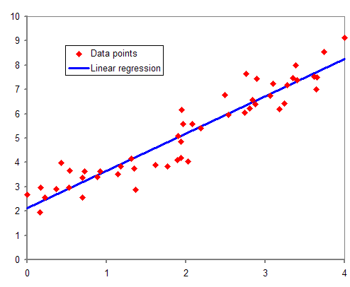
One of the most famous causal models is regression analysis. In statistical modeling, regression analysis is a set of statistical processes for estimating the relationships among variables. It includes many techniques for modeling and analyzing several variables, when the focus is on the relationship between a dependent variable and one or more independent variables (or ‘predictors’). More specifically, regression analysis helps one understand how the typical value of the dependent variable (or ‘criterion variable’) changes when any one of the independent variables is varied, while the other independent variables are held fixed.
Common Forecasting Assumptions:
- Forecasts are rarely, if ever, perfect. It is nearly impossible to 100% accurately estimate what the future will hold. Firms need to understand and expect some error in their forecasts.
- Forecasts tend to be more accurate for groups of items than for individual items in the group. The popular Fitbit may be producing six different models. Each model may be offered in several different colours. Each of those colours may come in small, large and extra large. The forecast for each model will be far more accurate than the forecast for each specific end item.
- Forecast accuracy will tend to decrease as the time horizon increases. The farther away the forecast is from the current date, the more uncertainty it will contain.
Demand Patterns
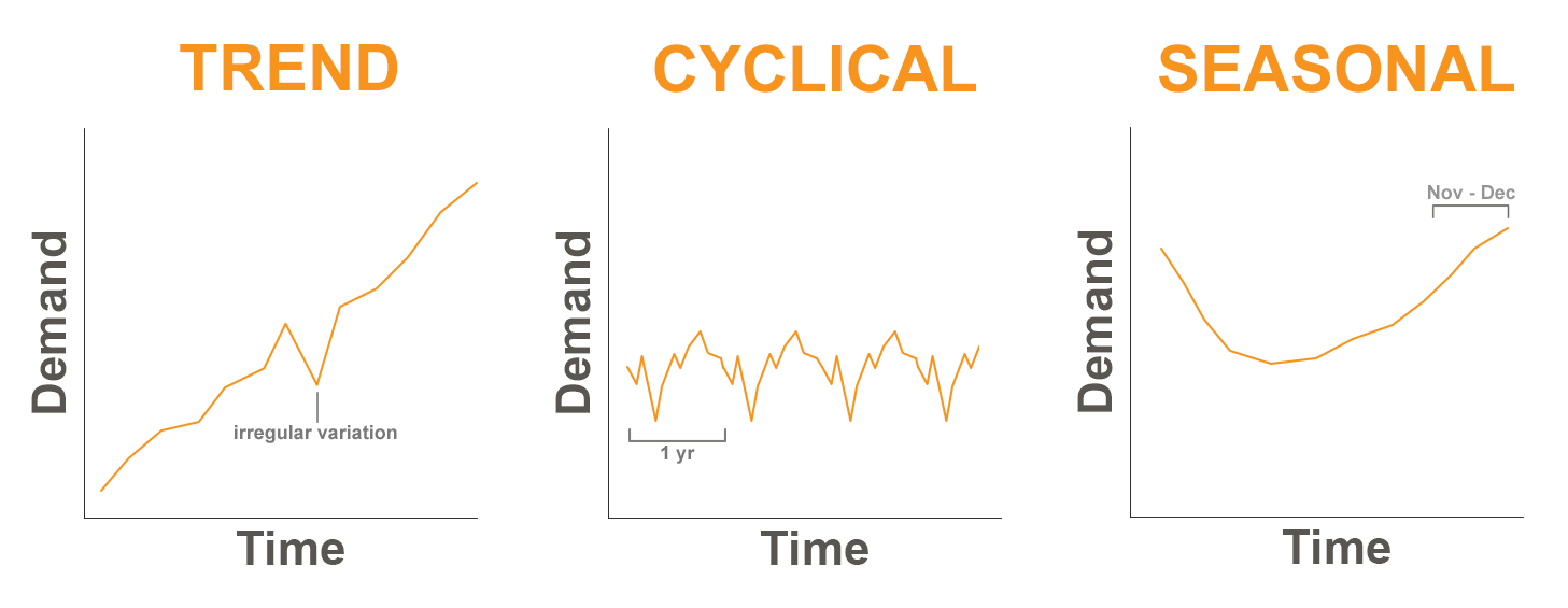
When we plot our historical product demand, the following patterns can often be found:
Trend – A trend is consistent upward or downward movement of the demand. This may be related to the product’s life cycle.
Cycle – A cycle is a pattern in the data that tends to last more than one year in duration. Often, they are related to events such as interest rates, the political climate, consumer confidence or other market factors.
Seasonal – Many products have a seasonal pattern, generally predictable changes in demand that are recurring every year. Fashion products and sporting goods are heavily influenced by seasonality.
Irregular variations – Often demand can be influenced by an event or series of events that are not expected to be repeated in the future. Examples might include an extreme weather event, a strike at a college campus, or a power outage.
Random variations – Random variations are the unexplained variations in demand that remain after all other factors are considered. Often this is referred to as noise.
Time Series Methods
Time series methods use historical data as the basis of estimating future outcomes. A time series is a series of data points indexed (or listed or graphed) in time order. Most commonly, a time series is a sequence taken at successive equally spaced points in time. Thus, it is a sequence of discrete-time data. Examples of time series are heights of ocean tides, counts of sunspots, and the daily closing value of the Dow Jones Industrial Average.
Time series are very frequently plotted via line charts. Time series are used in statistics, signal processing, pattern recognition, econometrics, mathematical finance, weather forecasting, earthquake prediction, electroencephalography, control engineering, astronomy, communications engineering, and largely in any domain of applied science and engineering which involves temporal measurements.[4]
In the following, we will elaborate more on some of the simpler time-series methods and go over some numerical examples.
Naïve Method
The simplest forecasting method is the naïve method. In this case, the forecast for the next period is set at the actual demand for the previous period. This method of forecasting may often be used as a benchmark in order to evaluate and compare other forecast methods.
Simple Moving Average
In this method, we take the average of the last “n” periods and use that as the forecast for the next period. The value of “n” can be defined by the management in order to achieve a more accurate forecast. For example, a manager may decide to use the demand values from the last four periods (i.e., n = 4) to calculate the 4-period moving average forecast for the next period.
Example
Some relevant notation:
Dt = Actual demand observed in period t
Ft = Forecast for period t
Using the following table, calculate the forecast for period 5 based on a 3-period moving average.
|
Period |
Actual Demand |
|
1 |
42 |
|
2 |
37 |
|
3 |
34 |
|
4 |
40 |
Solution
Forecast for period 5 = F5 = (D4 + D3 + D2) / 3 = (40 + 34 + 37) / 3 = 111 / 3 = 37
Here is a video explaining simple moving averages.
https://www.linkedin.com/learning/forecasting-using-financial-statements/simple-moving-average
Weighted Moving Average
This method is the same as the simple moving average with the addition of a weight for each one of the last “n” periods. In practice, these weights need to be determined in a way to produce the most accurate forecast. Let’s have a look at the same example, but this time, with weights:
Example
|
Period |
Actual Demand |
Weight |
|
1 |
42 |
|
|
2 |
37 |
0.2 |
|
3 |
34 |
0.3 |
|
4 |
40 |
0.5 |
Solution
Forecast for period 5 = F5 = (0.5 x D4 + 0.3 x D3 + 0.2 x D2) = (0.5 x 40+ 0.3 x 34 + 0.2 x 37) = 37.6
Note that if the sum of all the weights were not equal to 1, this number above had to be divided by the sum of all the weights to get the correct weighted moving average.
Here is a video explaining weighted moving averages.
https://www.linkedin.com/learning/forecasting-using-financial-statements/weighted-moving-average
Exponential Smoothing
This method uses a combination of the last actual demand and the last forecast to produce the forecast for the next period. There are a number of advantages to using this method. It can often result in a more accurate forecast. It is an easy method that enables forecasts to quickly react to new trends or changes. A benefit to exponential smoothing is that it does not require a large amount of historical data. Exponential smoothing requires the use of a smoothing coefficient called Alpha (α). The Alpha that is chosen will determines how quickly the forecast responds to changes in demand. It is also referred to as the Smoothing Factor.
There are two versions of the same formula for calculating the exponential smoothing.
Here is version #1:
Ft = (1 – α) Ft-1 + α Dt-1
Note that α is a coefficient between 0 and 1
For this method to work, we need to have the forecast for the previous period. This forecast is assumed to be obtained using the same exponential smoothing method. If there were no previous period forecast for any of the past periods, we will need to initiate this method of forecasting by making some assumptions. This is explained in the next example.
Example
|
Period |
Actual Demand |
Forecast |
|
1 |
42 |
|
|
2 |
37 |
|
|
3 |
34 |
|
|
4 |
40 |
|
|
5 |
|
|
In this example, period 5 is our next period for which we are looking for a forecast. In order to have that, we will need the forecast for the last period (i.e., period 4). But there is no forecast given for period 4. Thus, we will need to calculate the forecast for period 4 first. However, a similar issue exists for period 4, since we do not have the forecast for period 3. So, we need to go back for one more period and calculate the forecast for period 3. As you see, this will take us all the way back to period 1. Because there is no period before period 1, we will need to make some assumption for the forecast of period 1. One common assumption is to use the same demand of period 1 for its forecast. This will give us a forecast to start, and then, we can calculate the forecast for period 2 from there. Let’s see how the calculations work out:
If α = 0.3 (assume it is given here, but in practice, this value needs to be selected properly to produce the most accurate forecast)
Assume F1 = D1, which is equal to 42.
Then, calculate F2 = (1 – α) F1+ α D1 = (1 – 0.3) x 42 + 0.3 x 42 = 42
Next, calculate F3 = (1 – α) F2+ α D2 = (1 – 0.3) x 42 + 0.3 x 37 = 40.5
And similarly, F4 = (1 – α) F3+ α D3 = (1 – 0.3) x 40.5 + 0.3 x 34 = 38.55
And finally, F5 = (1 – α) F4+ α D4 = (1 – 0.3) x 38.55 + 0.3 x 40 = 38.985
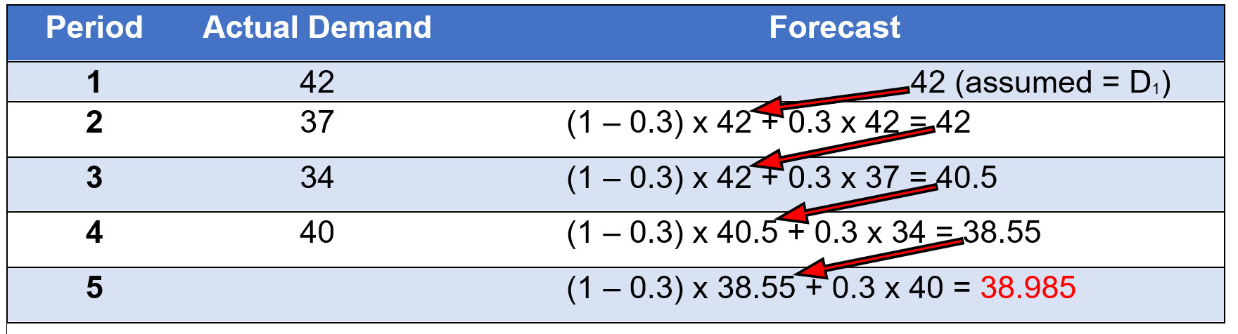
Accessible format for Figure 3.3
Here is a video explaining exponential smoothing using EXCEL.
https://www.linkedin.com/learning/search?keywords=exponential%20smoothing&u=2169170
Here is version #2:
Ft = Ft-1 + α(Dt-1 – Ft-1)
Example
Assume you are given an alpha of 0.3, Ft-1 = 55
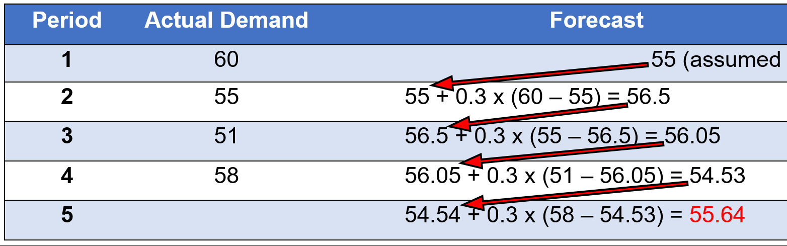
Accessible format for Figure 3.4
Seasonal Index
Many organizations produce goods whose demand is related to the seasons, or changes in weather throughout the year. In these cases, a seasonal index may be used to assist in the calculation of a forecast.
Example
|
Season |
Previous Sales |
Average Sales |
Seasonal Index |
|
Winter |
390 |
500 |
390 / 500 = .78 |
|
Spring |
460 |
500 |
460 / 500 = .92 |
|
Summer |
600 |
500 |
600 / 500 = 1.2 |
|
Fall |
550 |
500 |
550 / 500 = 1.1 |
|
Total |
2000 |
|
|
Using these calculated indices, we can forecast the demand for next year based on the expected annual demand for the next year. Let’s say a firm has estimated that next year annual demand will be 2500 units.
|
Season |
Anticipated annual demand |
Avg. Sales / Season |
Seasonal Factor |
New Forecast |
|
Winter |
|
625 |
0.78 |
.78 x 625 = 487.5 |
|
Spring |
|
625 |
0.92 |
.92 x 625 = 575 |
|
Summer |
|
625 |
1.2 |
1.2 x 625 = 750 |
|
Fall |
|
625 |
1.1 |
1.1 x 625 = 687.5 |
|
|
2500 |
|
|
|
Forecast Accuracy Measures
In this section, we will calculate forecast accuracy measures such as Mean Absolute Deviation (MAD), Mean Squared Error (MSE), and Mean Absolute Percentage Error (MAPE). We will explain the calculations using the next example.
Example
The following actual demand and forecast values are given for the past four periods. We want to calculate MAD, MSE and MAPE for this forecast to see how well it is doing.
Note that Abs (et) refers to the absolute value of the error in period t (et).
| Period | Actual Demand | Forecast |
et |
Abs (et) |
et2 |
[Abs (et) / Dt] x 100% |
| 1 | 63 | 68 | ||||
| 2 | 59 | 65 | ||||
| 3 | 54 | 61 | ||||
| 4 | 65 | 59 |
Step 1: Calculate the error as et = Dt – Ft (the difference between the actual demand and the forecast) for any period t and enter the values in the table above.
Step 2: Calculate the absolute value of the errors calculated in step 1 [i.e., Abs (et)], and enter the values in the table above.
Step 3: Calculate the squared error (i.e., et2) for each period and enter the values in the table above.
Step 4: Calculate [Abs (et) / Dt] x 100% for each period and enter the value under its column in the table above.
Solution
|
Period |
Actual Demand |
Forecast |
et |
Abs (et) |
et2 |
[Abs (et) / Dt] x 100% |
|
1 |
63 |
68 |
-5 |
5 |
25 |
7.94% |
|
2 |
59 |
65 |
-6 |
6 |
36 |
10.17% |
|
3 |
54 |
61 |
-7 |
7 |
49 |
12.96% |
|
4 |
65 |
59 |
6 |
6 |
36 |
9.23% |
Calculations for Accuracy Measures:
MAD = The average of what we calculated in step 2 (i.e., the average of all the absolute error values)
= (5 + 6 + 7 + 6) / 4 = 24 / 4 = 6
MSE = The average of what we calculated in step 3 (i.e., the average of all the squared error values)
= (25 + 36 + 49 + 36) / 4 = 146/4 = 36.5
MAPE = The average of what we calculated in step 4
= (7.94% + 10.17% + 12.96% + 9.23%) / 4 = 40.3/4 = 10.075%
Here is a video on Mean Absolute Deviation using EXCEL
https://www.linkedin.com/learning/search?keywords=mean%20absolute%20deviation%20&u=2169170
End of Chapter Problems
Problem #1
Below are monthly sales of light bulbs from the lighting store.
| Month | Sales |
| Jan | 255 |
| Feb | 298 |
| Mar | 357 |
| Apr | 319 |
| May | 360 |
| June |
.
Forecast sales for June using the following
- Naïve method
- Three- month simple moving average
- Three-month weighted moving average using weights of .5, .3 and .2
- Exponential smoothing using an alpha of .2 and a May forecast of 350.
Solution
- 360
- (357 + 319 + 360) / 3 = 345.3
- 360 x .5 + 319 x .3 + 357 x .2 = 347.1
- 350 + .2(360 – 350) = 352
Problem #2
Demand for aqua fit classes at a large Community Centre are as follows for the first six weeks of this year.
| Week | Demand |
| 1 | 162 |
| 2 | 158 |
| 3 | 138 |
| 4 | 190 |
| 5 | 182 |
| 6 | 177 |
| 7 |
.
You have been asked to experiment with several forecasting methods. Calculate the following values:
- a) Forecast for weeks 3 through week 7 using a two-period simple moving average
- b) Forecast for weeks 4 through week 7 using a three-period weighted moving average with weights of .6, .3 and .1
- c) Forecast for weeks 4 through week 7 using exponential smoothing. Begin with a week 3 forecast of 130 and use an alpha of .3
Solution
|
Week |
Demand |
a) |
b) |
c) |
|
1 |
162 |
|
|
|
|
2 |
158 |
|
|
|
|
3 |
138 |
(162 + 158) / 2 = 160 |
|
130 |
|
4 |
190 |
(158 + 138) / 2 = 148 |
138 x .6 + 158 x .3 + 162 x .1 = 146.4 |
130 + .3 x (138 – 130) = 132.4 |
|
5 |
182 |
(138 + 190) / 2 = 164 |
190 x .6 + 138 x .3 + 158 x .1 = 171.2 |
132.4 + .3 x (190 – 132.4) = 149.7 |
|
6 |
177 |
(190 + 182) / 2 = 186 |
182 x .6 + 190 x .3 + 138 x .1 = 180 |
149.7 + .3 x (182 – 149.7) = 159.4 |
|
7 |
|
(182 + 177) / 2 = 179.5 |
177 x .6 + 182 x .3 + 190 x .1 = 179.8 |
159.4 + .3 x (177 – 159.4) = 164.7 |
Problem #3
Sales of a new shed has grown steadily from the large farm supply store. Below are the sales from the past five years. Forecast the sales for 2018 and 2019 using exponential smoothing with an alpha of .4. In 2015, the forecast was 360. Calculate a forecast for 2016 through to 2020.
|
Year |
Sales |
Forecast |
|
2015 |
348 |
360 |
|
2016 |
372 |
|
|
2017 |
311 |
|
|
2018 |
371 |
|
|
2019 |
365 |
|
|
2020 |
|
|
.
Solution
|
Year |
Sales |
Forecast |
|
2015 |
348 |
360 |
|
2016 |
372 |
360 + .4 x (348 – 360) = 355.2 |
|
2017 |
311 |
355.2 + .4 x (372 – 355.2) = 361.9 |
|
2018 |
371 |
361.9 + .4 x (311 – 361.9) = 341.6 |
|
2019 |
365 |
341.6 + .4 x (371 – 341.6) = 353.3 |
|
2020 |
|
353.3 + .4 x (365-353.3) = 358.0 |
Problem #4
Below is the actual demand for X-rays at a medical clinic. Two methods of forecasting were used. Calculate a mean absolute deviation for each forecast method. Which one is more accurate?
| Week | Actual Demand | Forecast #1 | Forecast #2 |
| 1 | 48 | 50 | 50 |
| 2 | 65 | 55 | 56 |
| 3 | 58 | 60 | 55 |
| 4 | 79 | 70 | 85 |
Solution
|
Week |
Actual Demand |
Forecast #1 |
IerrorI |
Forecast #2 |
IerrorI |
|
1 |
48 |
50 |
2 |
50 |
2 |
|
2 |
65 |
55 |
10 |
56 |
9 |
|
3 |
58 |
60 |
2 |
55 |
3 |
|
4 |
79 |
70 |
9 |
85 |
6 |
|
|
|
Mean Abs Deviation: |
5.75 |
Mean Abs Deviation: |
5 |
- Wikipedia contributors. (2019). Forecasting. In Wikipedia, The Free Encyclopedia. Retrieved November 4, 2019, from https://en.wikipedia.org/w/index.php?title=Forecasting&oldid=933732816 ↵
- Saylor Academy. (2012). Principles of Marketing. Forecasting. Retrieved on November 4, 2019, from https://saylordotorg.github.io/text_principles-of-marketing-v2.0/s19-03-forecasting.html ↵
- Wikipedia contributors. (2019). Forecasting. In Wikipedia, The Free Encyclopedia. Retrieved on November 4, 2019, from https://en.wikipedia.org/w/index.php?title=Forecasting&oldid=933732816 ↵
- Wikipedia contributors. (2019). Time series. In Wikipedia, The Free Encyclopedia. Retrieved on November 4, 2019, from https://en.wikipedia.org/w/index.php?title=Time_series&oldid=934671965 ↵
