8 Inventory Management
Introduction
In this chapter, we are going to talk about inventory management models that deal with certain or known demand. The basic questions that any inventory management model tries to address are 1) how many units to order, and 2) when to place the order for those units. The objective of any inventory control or inventory management is to achieve satisfactory levels of customer service while keeping inventory costs reasonably low. So, there’s always a trade-off between how much inventory you keep versus the level of customer service that you provide.
Types of Inventory
There are several types of inventory in any organization. Here are some that are more common:
– Raw materials or purchased parts are some of the very common types.
– Work in process (or progress) or WIP, which are the semi-finished or not completely finished items that you can find in the middle of assembly lines and manufacturing facilities.
– Finished goods or merchandise that we’re all familiar with. We can find these in all the stores that we go to buy what we need.
– Spare parts or tools and supplies are also another type of inventory that companies may need basically
Reasons for Keeping Inventory
There are different reasons for keeping or holding inventory. Here are some examples:
– To hold inventory simply because that inventory is still in transit. In that case, it has not got to their facility yet and because they have paid for those items, they are counted as their inventory and this is something that we also call in transit inventory holding.
– To protect against the stock outs. This is a very common or probably the most common reason for keeping inventory. That is, when the customers come to ask us for a unit of product to purchase, we want to make sure that we have enough in stock.
– To take advantage of some quantity discounts that might be available to us by our suppliers. What happens is that our suppliers may tell us that if we purchase more, they will be able to give us some discounts. Note that we did not necessarily need the extra units at this time. As a result, we will need to keep them in stock and that will be our extra inventory to hold. We’re going to talk about the discount model in this video as well and over there, you’ll see what kinds of trade-offs are there and in which scenario it is better to take advantage of some discount versus not.
– To smooth out the production requirements. This simply means that from time to time, if the demand goes up and down, when the demand is down, you may want to produce a little bit more and keep it in inventory, so that later on, when the demand goes back up, you don’t have to necessarily ramp up your production too much. But instead, you can use the inventory that you have piled up. This helps you keep a more steady production level at all times, which is usually a less costly way of doing the production.
– To cover for any disruption in the operations. This means if anything goes wrong in a certain part of a production process, you will have enough inventory around to cover you for that part of the operation. This way, you will most likely not have to shut down the whole production line, or you can at least delay the shutdown as much as possible, until the problem gets resolved.
Please note that in any of these scenarios, we will need to pay a close attention to the holding costs of the inventory versus the other costs. For example, if the inventory holding cost is very high, we may prefer to have a potential stockout sometimes as opposed to keeping a lot more inventory in stock. In another example, we may not use the discount option from our supplier if we know that the total savings (as a result of the discount) is not worth the additional inventory holding costs. We will discuss more about the inventory holding costs later in this chapter.
Inventory Management Models
Generally speaking in inventory management, we look at the demand as an either known or more steady demand versus uncertain demand. We also have other factors to impact the type of model used. Lead time is one of these factors. Lead time is defined as the time from when you place an order to a supplier until you receive that order. Another factor is the review time. Review time is referring to how you review your inventory levels. For example, one method is called continuous review, which means that your information system will automatically check your inventory level at all times and when the inventory level hits a certain point, which we call the reorder point, the system will notify us that we need to place an order or even in more automated systems the system may automatically place the order and that way, we do not have to do anything. The order will automatically be placed to the supplier that we have an agreement with already.
Another type of review method that we have is called periodic review or fixed order interval. In this method, we check the inventory level at the end of certain fixed order intervals and if our inventory is less than a certain maximum level (which we can optimally determine beforehand), we will calculate how much difference is there, and we will place an order for that amount.
There are also other factors to be considered which we are not going to go into that much detail of those things here. For example, if there is any perishability or obsolescence, especially for items like food that can get perished. If so, that can make the inventory models a bit more complicated. In that case, we should consider the life span of the product that is perishable to make sure that we are not bringing in too much, or otherwise, it will be perished or obsolete, and the whole thing would be a total waste of our money.
Relevant Costs
The costs are usually defined for each item or stock keeping unit (SKU) separately. As a result, the optimal order quantities and the time of order is determined for each item specifically. The relevant costs that we have in any inventory management are as follows:
– Total Purchasing or Acquisition Cost:
This refers to the total purchasing cost of an item in a year (or in a month or a quarter of the year, etc., depending on what our unit of measure is for the time). In some models, this particular cost may not change. This is because the total demand in the year is the same (in those models) and if the price is not changing (that is, there’s no quantity discount available from the supplier), the total acquisition cost or purchasing cost will be fixed. As a result, in those scenarios, we ignore this cost from our mathematical model, since we are doing our calculations to find the optimal order quantities and because this is a fixed cost and it does not change based on how much we order every single time, the total acquisition cost or purchase cost in the year will stay fixed.
– Total Ordering Costs:
Ordering cost usually includes the clerical and retrieval expenses. Sometimes, we include the delivery and inspection a part of this cost too. If you have your own manufacturing (instead of buying from an outside supplier), this same cost will be called setup cost which we have it in the model that we call Economic Production Quantity (EPQ).
– Total Carrying or Holding Costs:
This refers to the total cost of holding the items as if they were kept in stock for a whole year. Since each item will usually not stay in stock for the whole year, if we are to calculate the total annual holding cost, we will need to find an average number of items that we can find in our stock every time that we check our inventory. For example, if we checked our inventory level for a certain item 20 times during a year, we would most likely get a different number every time. If we take the average of those 20 numbers, that will give us a good estimate of how many units are sitting in our warehouse at all times. Please note that the items come in and go out of our facility as we buy and sell (or use) them. So, the items that we see on the stock each time are not necessarily the same ones sitting there for so long.
The unit holding cost is defined as cost of holding one unit of product for one unit of time. The unit of time is usually one year. But it can be based on a quarter, month, day or any other time unit. The key is to be consistent with the unit of measurement for time wherever in our calculations.
In operations management, we usually calculate the holding cost for each item as a percentage of the item’s value. For example, if the value of the item that we are keeping in stock is $1000 and our inventory holding cost is 20%, this means that if we keep that item for one whole year, it will cost us 20% x 1000 = $200 per unit. If the same item sits in our inventory for only a quarter of the year, it will cost of (1/4) x 200 = $50 per unit. If we had 10 of this item and they were kept for one whole year, the total annual inventory holding cost would be 10 x 200 = $2000.
Insight:
“If the price or the value of the item is higher, the holding cost will be higher. That is one of the main reasons that when companies are dealing with more expensive items, they tend to keep as few units as possible for those items. Sometimes, they keep only one unit just for showing at their store, and they get the customers’ orders to deliver the item to them later, or to bring it to the store for customers’ pickup later. They could not afford keeping several of those very expensive items in the store, because otherwise, the cost of holding them would be very high.”
The holding cost percentage represents all the costs associated with the facility in which the item is kept as well as any material handling costs within the facility. Basically, you will need to talk to the accountants in our company, if you are in charge of inventory, to get a better sense of the costs and a better idea of this percentage. In this chapter, we will have this percentage given to us in any examples that we have.
Some of the costs included in the holding cost percentage are as follows:
- Cost of capital
This means that when your money is tied to the inventory that you are keeping, you cannot invest that money anywhere else. So, you are losing some sort of an opportunity out there. As a result, the estimation of an interest that you could have gained can give us a percentage which is used as a part of the holding cost percentage.
- Insurances
Since we always need to have insurance for our warehouses, the cost of insurance can be calculated as a percentage for each item. This cost will in turn be used as another part of holding cost percentage.
- Storage costs
As share of the actual cost of owning or leasing the warehouse or the facility in which we hold the inventory and the costs of running the place (e.g., material handling, utilities, etc.) are calculated per item and added to the holding cost percentage.
- Breakage or spoilage
If there is any breakage, theft or spoilage that happens to our stock from time to time, we will need to add that as an additional part of the holding cost.
– Shortage Costs
There could be some penalty or shortage costs if there were uncertainties in the demand. If the demand were higher than what you have available in your inventory, you would have a shortage. This cost is usually a tricky one, since it does not look like a cost for which you lose money out of your pocket right away. But in fact, you are not gaining the money that you could make if you had enough units of the item in demand available. You can also lose the sale to certain customers completely, as they may find substitute products from other companies. In addition, there is a chance for a loss of goodwill in our customers, specially if the shortage happens over and over again. In all these cases, the inventory management tries to monetize the amount of loss to plan more properly for an optimal level of product availability.
Inventory Models for Certain Demand: Economic Order Quantity (EOQ)
The very first model that we want to talk about is the simplest model out there, and is called Economic Order Quantity or EOQ. This model is very famous and the assumptions or conditions under which it works are as follows:
– We are ordering the product or item from an outside supplier. That is, we do not have our own production of the item.
– The demand is fixed or steady per unit of time (e.g., per year). Because the demand is fixed or known, there’s no reason to have a shortage. Basically, it means that you know exactly how much money you are going to make if you bring in enough number of units to satisfy that demand.
– The lead time is constant. That is, there is no uncertainty because of the lead time either. So, if your supplier tells you that they are going to deliver in five days, you can certainly assume that five days is exactly five days and it is not going to be seven or it is not going to be three or four either.
– We order a fixed amount or the same amount every time that we place an order to our supplier.
– Our ordering cost is a fixed cost per order. Sometimes, when we order a greater number of units, our ordering cost per unit may change. But here, we are assuming that the ordering cost per order is simply the cost of administration in terms of placing the order and putting together the paperwork, etc. So, this simply means that if we order a larger or smaller lot size, it will not affect our ordering cost for that one order. But, it will change the number of orders that we place in a year. For example, if we order a larger lot size every time (note that all orders throughout the year are equal in size, based on the previous assumption), we will end up placing fewer number of orders in a whole year, and that will result in our total ordering cost in a year going down.
Inventory Control Cycles or Order Cycles
Usually, every order is associated with what we call an order cycle. We place an order and the order comes in, and then, we use the order that has come in to satisfy the demand, and then later on, when our inventory level gets down to a certain level, we place another order and after that, the same things get repeated again and again. That’s why every one of these is called a cycle which gets repeated.
The picture below shows how the inventory level can change during the time:
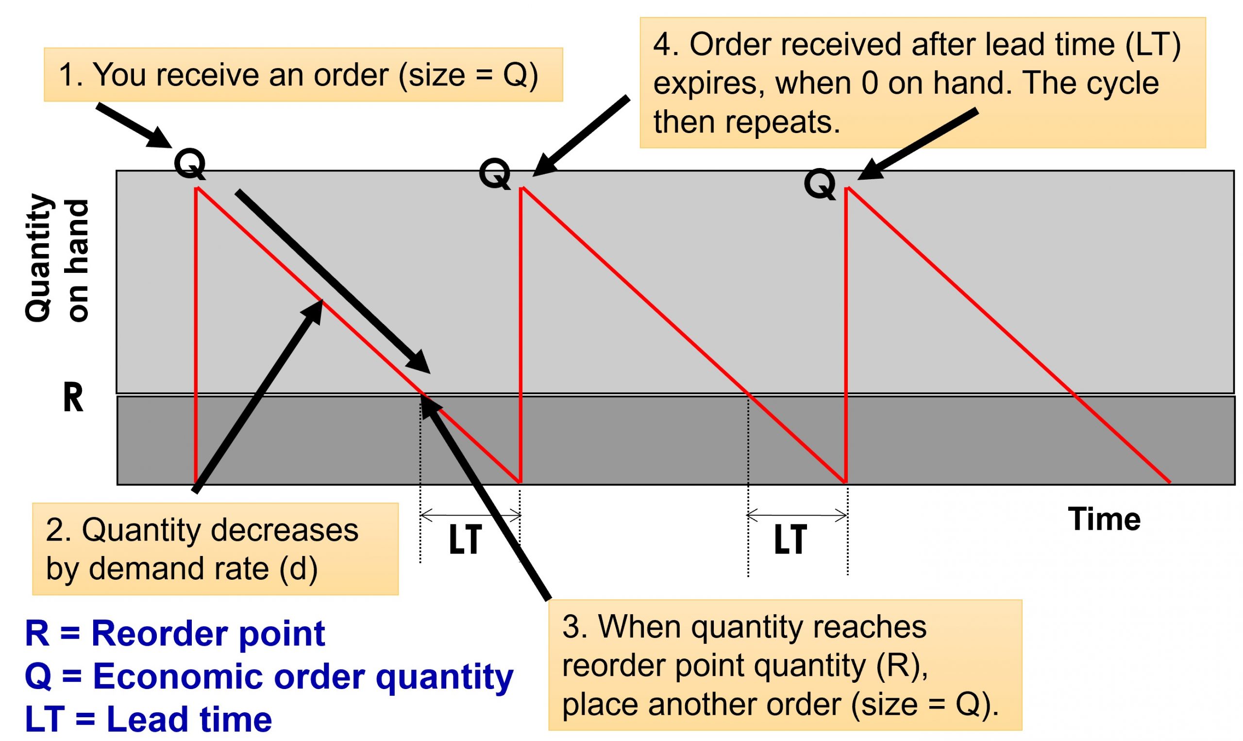
The vertical axis is showing us the inventory level on hand, and the horizontal the time. The red line is showing the inventory level. At point #1, we receive an order. That is why our inventory level jumps up all the way from zero to Q units (Note that in the EOQ model, we order Q units every time we place an order to our supplier). As time passes (which is from left to right), the inventory level goes down due to the customer demand that we are satisfying from the inventory that we have on hand. Then, our inventory level gets to a certain point that we call R or reorder point. That is exactly the time that we need to place our next order.
Because we do not want to have shortages, we consider a period of time which is equal to lead time and we go back in time for that amount (i.e., the duration of lead time) from when we expect our inventory level to hit zero, and we place the order right then. This way, we will have just enough inventory from when we place the order, which is at the reorder point, until the end of lead time, which is when our inventory is expected to hit zero, and exactly when we expect to receive our order.
The only reason that we can do this with such confidence is that as mentioned before, the demand rate is fixed. As a result, we know exactly how the demand is changing and how much ahead of the time we need to place this order so that we received it just as we are about to run out. The time from when the order comes in until when the next order is received is called cycle time.
The EOQ Model Calculations
The objective of the EOQ model is to find the optimal order quantity (the size of the order that we place each time) which can minimize our total costs. As mentioned under the section for relevant costs earlier in this chapter, some costs may not be included in the calculations for different reasons. For example, the total acquisition (purchasing) cost is not included in the EOQ model without discounts, because that total amount stays the same no matter what order size we use throughout the year. We discussed this earlier. In addition, some costs like the shortage cost are not included because the assumptions or conditions behind the EOQ model will automatically result in no shortage. As a result, there will not be any shortage to consider.
The only costs that are applicable to the EOQ model are the total ordering cost and the total inventory holding (carrying) cost. In our calculations in the following, we will calculate these costs for one whole year, and our goal is to minimize the sum of these costs in a year by finding the optimal order quantity.
Here are the notations and some basic calculations:
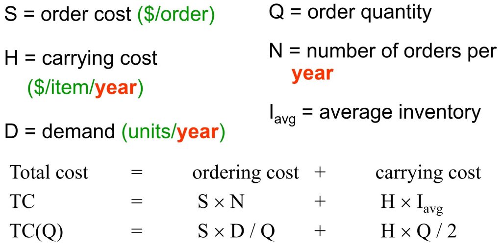
Note that S is the fixed order cost per order. N which is the number of orders per year can easily be calculated. We know that in total, we need a demand of D units to satisfy in a year and we also know that we are bringing in Q units each time. For example, if the demand is 1000 units per year and if you order quantity happened to be 100 units, we will need to place our order 10 times throughout the year, which is 1000/10.
About the average inventory, as mentioned in the section on relevant costs earlier in this chapter, we use the average inventory level to represent the inventory that we can see in our facility at all times during the year. That is why we multiply that by H which is the cost of holding one unit of inventory for one whole year. Please note that as mentioned before, the time measurement unit does not have to be in years. But if we needed to use a different time unit, we will need the other parts of the calculations (in this case, the demand) to be consistent with it to make sure they are all defined based on the same time unit of measurement.
Since we want to minimize the total cost by finding the optimal order quantity, we will need to use the function that we have for it (called TC(Q) here) and find the value of the Q that makes the derivate of this function equal to zero. Assuming that we have done all that, the final result is as follows:
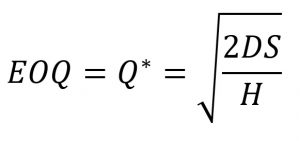
The * on top of Q shows that it is a special value of the Q, in this case, the optimal value. Let’s have a look at some examples.
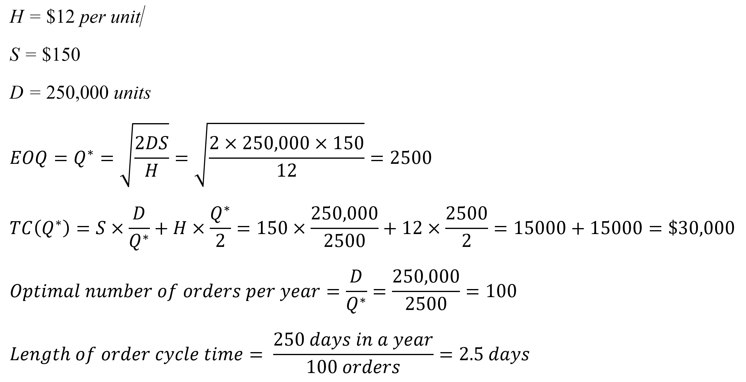
Example 1
Assume that Apple Canada has an annual demand of 250,000 for one of its tablets. A component has annual holding cost of $12 per unit, and ordering cost of $150. Calculate EOQ, total cost of ordering and inventory holding, number of orders per year and the order cycle time for this item. Assume 250 working days in a year.
Solution:
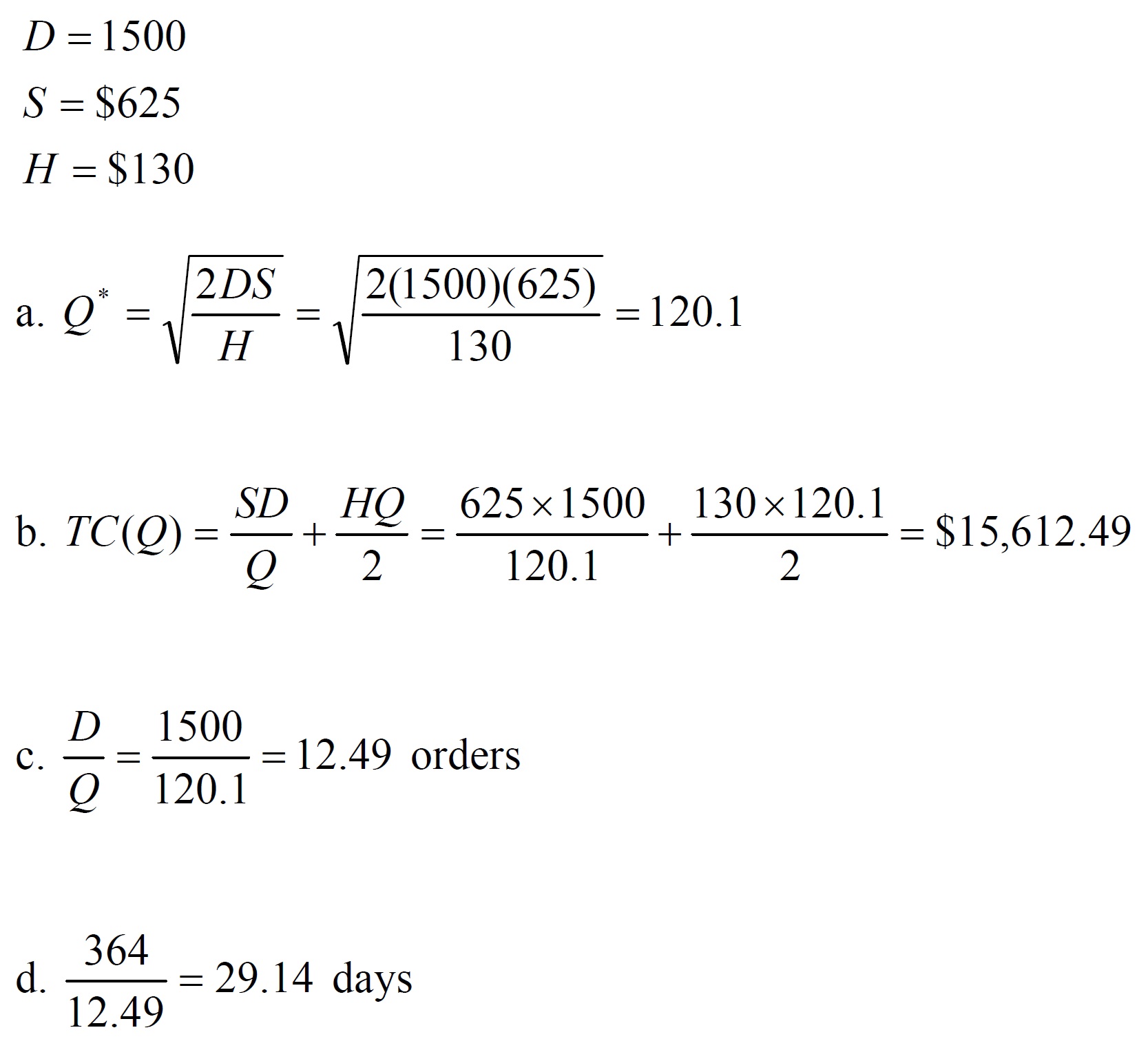
Example 2
Assume that it costs BestBuy $625 each time it places an order with a manufacturer for a specific model of laptop. The cost of carrying one laptop in inventory for a year is $130. The store manager estimates that total annual demand for the laptops will be 1500 units, with a constant demand rate throughout the year. The store policy is never to have stockouts of the laptops. The store is open for business every day of the year except Christmas Day.
Determine the following:
a. Optimal order quantity per order
b. Minimum total annual inventory costs
c. The optimal number of orders per year
d. The time between orders (in working days)
Solution:
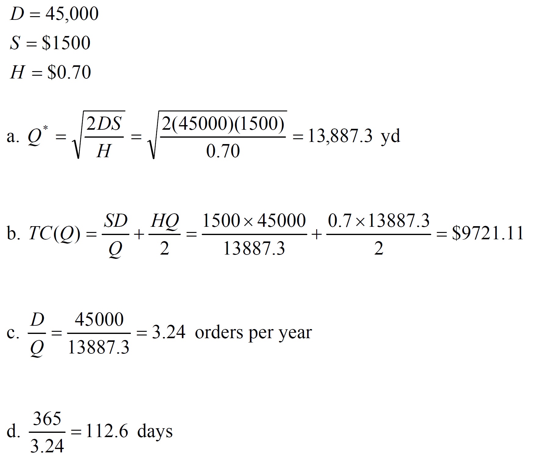
Example 3
The Modern Furniture Company purchases upholstery material from textile supplier in Halifax, Canada. The company uses 45,000 yards of material per year to make sofas. The cost of ordering material from the textile company is $1500 per order. It costs Modern Furniture $0.70 per yard annually to hold a yard of material in inventory. Determine:
a. The optimal number of yards of material Modern Furniture should order
b. The minimum total inventory cost
c. The optimal number of orders per year, and
d. The optimal time between orders
Solution:
Inventory Models for Certain Demand: Economic Production Quantity (EPQ)
The second model that we have for certain or known demand scenarios is called Economic Production Quantity. In this model, we do not order from an outside supplier. Instead, we have our own production. As a result, we have a production setup cost since we will need to setup the machines or the production area before the start of the production in each cycle. In addition, having a production makes receiving of the items in our stock more gradual. This is as opposed to the sudden receiving of Q units in the EOQ model. Thus, there is a slight change to the formulations compared to the EOQ model. The following graph shows how the inventory level changes through time in the EPQ model:
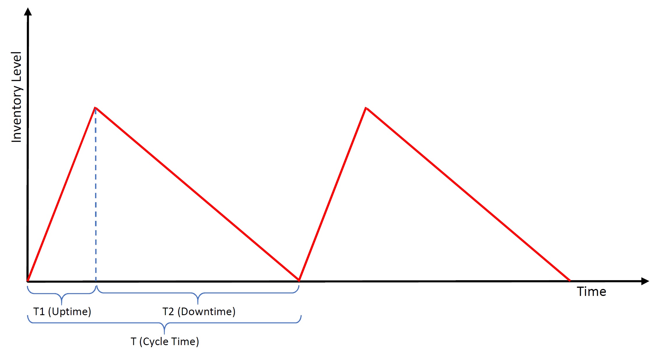
The red line is showing the inventory level. During the uptime or run time (T1) we are running the production with a rate of p per day while the demand is happening with a rate of d per day. As a result, the inventory level increases with a rate of p – d. We continue the production until our inventory is piled up to a certain maximum level. Then, we stop the production, and only use the piled-up inventory to satisfy the customer demand. This period is called downtime (T2). The basic assumption here is that the production rate is larger than the demand rate. Otherwise, we will always have a shortage.
In terms of calculations, if we use the following notation and replace the H (i.e., the holding cost per unit of item per year) by it, we can use the same formulations from the EOQ model for the optimal lot size (run size) and the total cost. Here are the calculations:
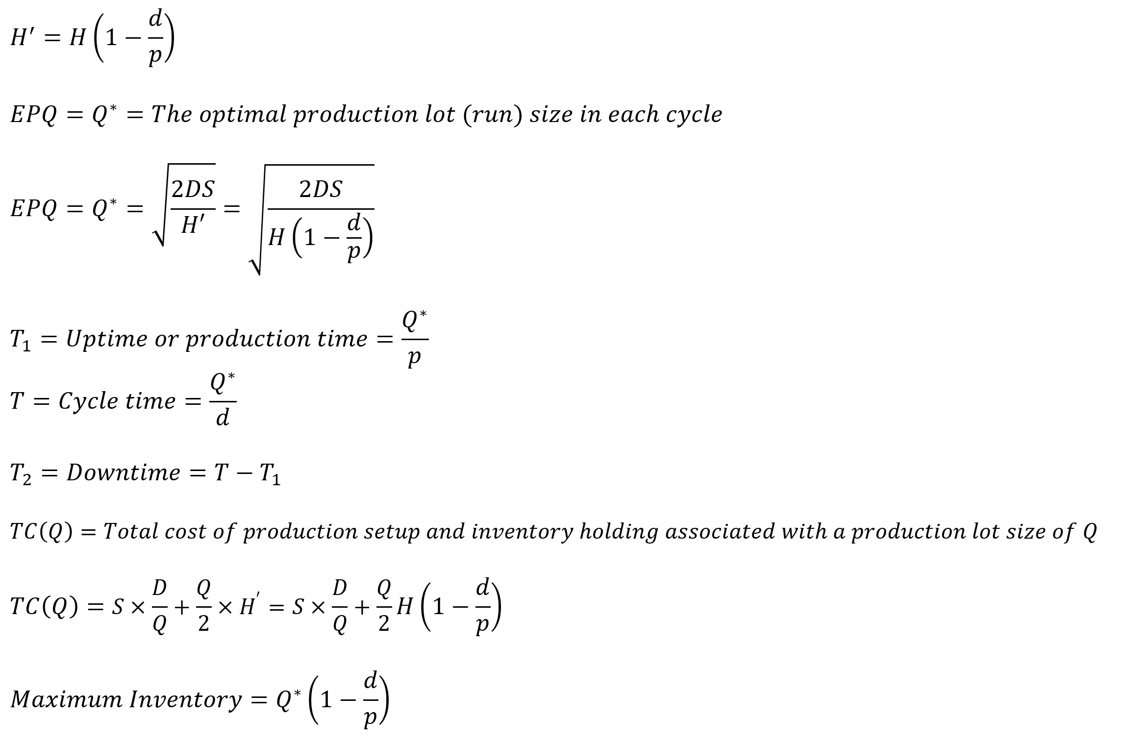
Note that “D” is defined as the demand per year, while “d” is the demand per day. In addition, Q* is a specific value for Q, which is associated with the optimal quantity. If we need to find the optimal total cost, we will need to use the value of Q* as the Q in the formula for TC(Q). Let’s have a look at an example.
Example 4
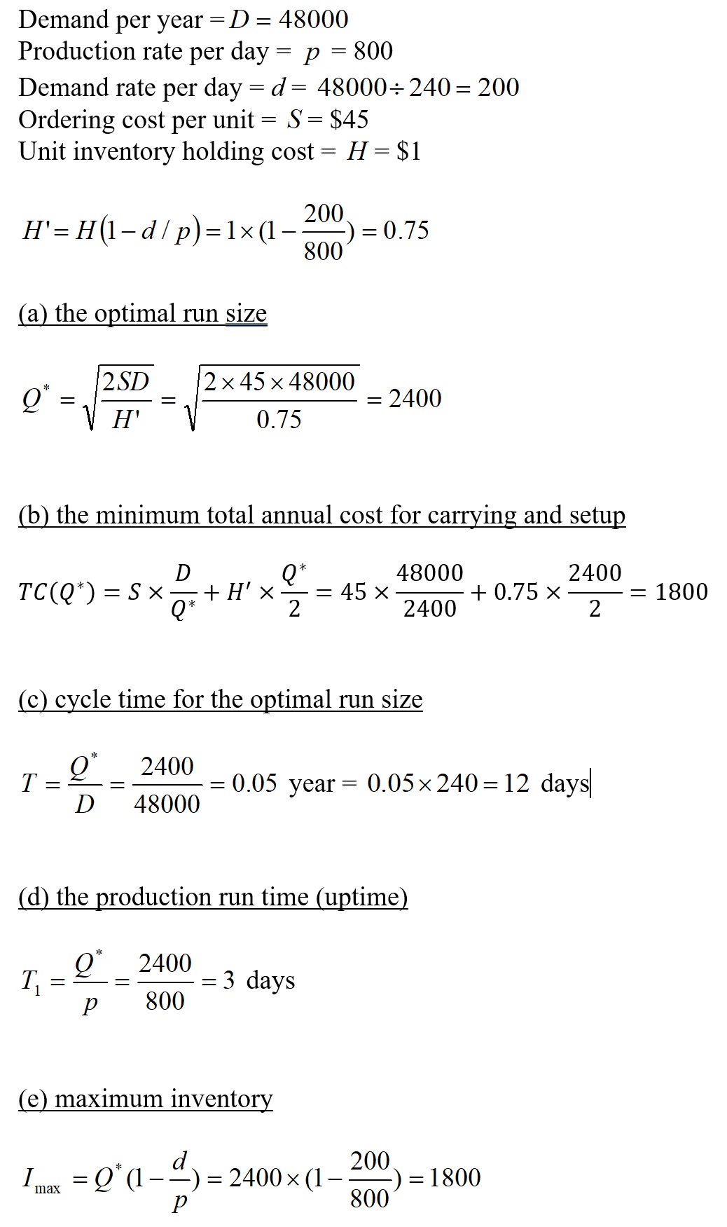
An automotive manufacturer uses 48,000 M1 gearboxes per year for its X1 SUV series. The firm makes its own M1 gearboxes, which it can produce at a rate of 800 per day. Carrying cost is $1 per gearbox per year. Setup cost for a production run of M1 gearboxes is $45. The firm operates 240 days per year. Determine:
a. the optimal run size,
b. the minimum total annual cost for carrying and setup,
c. cycle time for the optimal run size,
d. the production run time (uptime), and
e. maximum inventory.
Solution: